In recent years, computational chemistry has become an increasingly powerful tool for exploring the properties of materials at the molecular level. However, these techniques can often be challenging to implement, requiring specialized software and expertise in computational methods. In this blog post, I'll show you how to run quantum mechanical simulations of single-walled carbon nanotubes filled with small molecules using the open-source software packages ASE and Quantum ESPRESSO.
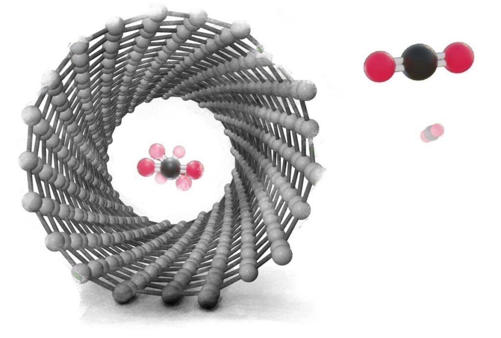
Before we dive into the code, let's first discuss what we're trying to simulate. Carbon nanotubes are cylindrical structures made entirely of carbon atoms, and they have unique mechanical, electrical, and thermal properties. By filling these nanotubes with small molecules, we can explore how the presence of these molecules affects the properties of the nanotube or how molecules behave inside it.
Create a folder where you want to run your simulations. This is where you will have your input and output files plus all the temporary files generated during the calculations. Open your text editor of choice (I use neovim, but you can use the one you prefer). Firstrly we import the modules we need to use.
import numpy as np
from ase.build import nanotube
from ase.build import molecule
from ase.build.attach import attach
from ase.io import  write
from ase.visualize import view
from ase.constraints import FixAtoms
from ase.calculators.espresso import Espresso
To get started, we need to define the parameters of our system. In this example, we will use carbon dioxide (CO2) molecules, but you could substitute other molecules depending on your research interests. We will also specify the size of the nanotube, the number of molecules to fill it, and the compression factor that determines how close together the molecules will be placed inside the nanotube.
# ---------------------------
# System Geometry parameters
# ---------------------------

# Molecules
molec = 'CO2'
N_molecules = 2
compresion_factor = 1.0  # How close the molecules will be inside the CNT
Now we set the properties of the carbon nanotube. We will use the nanotube() function, which takes as arguments the nanotube vectors (n, m) and the length of the nanotube. Also, we set the distance between neighbour CNT (as we will be running 3D periodic systems).
# CNT
cnt_n, cnt_m = 8, 0  # n,m nanotube vectors
cnt_l = 1   # Repetition units of a single CNT
cnt_gap = 4 # Distance betwen CNTs (Ang)
We can continue building the system using the ASE package. We create the small molecules using the molecule() function and attach them to the nanotube using the attach() function. We will rotate the molecules for them to be perpendicular to the longitudinal axis of the CNT. We also define constraints to keep the carbon atoms of the nanotube fixed in place during the simulation using the FixAtoms() function.
# ---------------------------
# Build the System
# ---------------------------

# CNT
cnt = nanotube(cnt_n,cnt_m, length=cnt_l)

def get_xy_distance(a,b):
    """
    Calculates the distance between 2 vectors in their projections on the XY plane (ignores the Z coordinate)
    """
    return np.linalg.norm(a[0:2] - b[0:2])

# Get the limits of the CNT
cnt_xyz = cnt.get_positions()
min_x, max_x =  min(cnt_xyz[:,0]), max(cnt_xyz[:,0])
min_y, max_y =  min(cnt_xyz[:,1]), max(cnt_xyz[:,1])
min_z, max_z =  min(cnt_xyz[:,2]), max(cnt_xyz[:,2])
cell_z = cnt.get_cell()[2][2]

# Used to arrange the molecules along the Z axis of the CNT
molecular_distance_z = cell_z/N_molecules * compresion_factor

# Attach the molecules
molecules = molecule(molec)
molecules.rotate(90,'x')
mmol = molecule(molec)
mmol.rotate(90,'x')
for m in range(1,N_molecules):
    mmol.rotate((360/N_molecules * m),'z')
    molecules = attach(molecules,mmol, distance=molecular_distance_z,  direction=(0,0,1))

constraints = FixAtoms(mask=[atom.symbol == 'C' for atom in cnt])
cnt.set_constraint(constraints)

# Add the CNT to the molecular system
system = cnt + molecules      # It does preserve constraints

# Set cell
cell_x = [(max_x - min_x + cnt_gap), 0, 0 ]
cell_y = [0, (max_y - min_y + cnt_gap), 0 ]
cell_z = cnt.get_cell()[2]  # Use the lattice parameter Z of the CNT
system.set_cell([cell_x,cell_y, cell_z])
After building the system, we set up the calculation parameters, including the energy cutoff, convergence criteria, and pseudopotentials. These are all specified in the input_params dictionary, which is then passed to the Quantum ESPRESSO calculator object. Finally, we run the calculation and retrieve the total energy of the system using the get_total_energy() method.
# ---------------------------
# Calculation parameters
# ---------------------------

input_params = {
               "ecutwfc": 45,       # plane-wave wave-function cutoff
               "ecutrho": 180,     # density wave-function cutoff,
               "conv_thr": 1e-6,  # DFT self-consistency convergence
               "pseudo_dir": "/home/user/pseudos/qe/SSSP_1.1.2_PBE_precision/", #  pseudo potentials directory
               "occupations": 'smearing',   #  Add smearing
               "smearing": 'cold',   # kind of smearing
               "degauss": 0.02,    # Amount of smearing
               "tprnfor": True,       # Print the forces
               "tstress": True,       # Print the stress tensor
               "vdw_corr": 'xdm'   # Use xchange-dipole moment van der Waals correction
               }
# Another way of adding a new paramter to the input_params dict
input_params["calculation"] = 'scf'

# define the pseudopotentials ( the 'pseudo_dir' path has to exist in your system)
pseudos = {"C": "C.pbe-n-kjpaw_psl.1.0.0.UPF",
           "O": "O.pbe-n-kjpaw_psl.0.1.UPF" }

kpts = (1, 1, 1)-
ecutwfc: This parameter sets the plane-wave energy cutoff used for the wave functions. A higher value leads to a more accurate solution, but it also requires more computational resources.
-
ecutrho: This parameter sets the plane-wave energy cutoff used for the charge density.
-
conv_thr: sets the convergence threshold for the self-consistent field iteration. It determines how close the electronic structure is to the true solution. A lower value leads to a more accurate solution, but it also will take longer for the calculation to converge.
-
pseudo_dir: sets the path where the pseudopotential files are stored. It has to point to the path in your system where you have downloaded the required pseudopotentials.
-
occupations: This parameter specifies how the occupation of the electronic states is determined. In this case, 'smearing' is used to smooth the electronic distribution, avoiding numerical instabilities.
-
smearing: This parameter specifies the kind of smearing to be used. In this case, 'cold' is the Marzari-Vanderbilt-DeVita-Payne cold smearing.
-
degauss: This parameter sets the width of the smearing function. A higher value leads to a smoother electronic distribution, but it also leads to a less accurate solution.
-
tprnfor: This parameter specifies whether the forces acting on each atom in the system are printed during the simulation. This is useful for debugging purposes and for understanding the behavior of the system.
-
tstress: This parameter specifies whether the stress tensor (which describes the mechanical stress on the system) is printed during the simulation. This is useful for understanding how the system responds to external perturbations.
Now it is time to check that our system looks like what we want to calculate:
# ---------------------------
# Visualize the system
# ---------------------------

# This is the initial system
view(system);
If all looks correct it is time to run the calculation. Note that we've set some constraints to the CNT, but as we are going to run a single point calculations, those constraints will not have any effect. The constraints only would be relevant if we are doing an optimization of the geometry, and for that you will need to set the calculation parameter of the input_params to 'relax'. But that would be a more expensive calculation that you can run once this one is properly working.
#------------------------
# Run the calculation
#------------------------

calc_QE = Espresso(input_data=input_params, pseudopotentials = pseudos, kpts=kpts)
system.set_calculator(calc_QE)
system.get_total_energy()
Save your file, with a name of your choice, like CO2_in_CNT.py. To run the calculation you have to execute this script with python:
python3 ./CO2_in_CNT.py
At the end of the calculation, you should have two new files in your folder : espresso.pwi (input file) and espresso.pwo (output file) plus a folder containing the temporary files generated during the sumulation.
If you want to use all the cores of your machine, you can even use mpiexec (if you have it installed when you installed the required packages) and use multiple cores.
mpiexec -np 4 python3 ./CO2_in_CNT.py
where -np 4 indicates the number of processors you want to use.
The code I've provided here is a simplified example, as I have not talked about parameter optimization, but it should give you an idea of how to get started with your own simulations. With ASE and Quantum ESPRESSO, you have a powerful set of tools at your disposal for exploring the properties of materials at the molecular level. And best of all, these tools are open-source and freely available, making them accessible to anyone with an interest in computational chemistry.
Installation of required packages
Install conda: If you don't have conda installed, you can download it from https://docs.conda.io/en/latest/miniconda.html and follow the installation instructions.
Create a new conda environment: Open a terminal window and create a new conda environment using the following command:
conda create --name nanotube_simulations python=3.9
This command will create a new environment named nanotube_simulations with Python version 3.9. You can choose any other name or Python version that suits your needs.
Once the environment is created, activate it using the following command:
conda activate nanotube_simulations
This command will activate the nanotube_simulations environment.
Install the required packages: You can also install numpy, matplotlib or any other package that you need for your project.
conda install -c conda-forge ase jupyterlab numpy
Install Quantum Espresso: Install Quantum Espresso following the instructions provided on their website: https://www.quantum-espresso.org/. Alternatively, you can also install it using conda with the following command:
conda install -c conda-forge qe
This command will install the Quantum Espresso package from the conda-forge channel.
With these steps, you should have all the required packages installed and be able to run the simulation code.
I hope this blog post has been informative and helpful. If you have any questions or feedback, please don't hesitate to leave a comment below. Happy.simulating()